Proximal Policy Optimization Family#
Proximal Policy Optimization: A Recap#
Preliminary:
Vanilla Policy Gradient (PG)
Trust Region Policy Optimization (TRPO)
General Advantage Estimation (GAE)
Proximal Policy Optimization (PPO) is a simple first-order optimization algorithm for reinforcement learning. It is similar to another algorithm called Trust Region Policy Optimization (TRPO) but with a simpler implementation. The PPO algorithm defines the probability ratio between the new policy and the old policy as \(\frac{\pi_{\theta}(a|s)}{\pi_{\theta_k}(a|s)}\) where \(\theta\) is the new policy and \(\theta_k\) is the old policy. Instead of adding complicated KL constraints, PPO ensures that this policy ratio stays within a small interval between \(1-\epsilon\) and \(1+\epsilon\), where \(\epsilon\) is a hyperparameter that controls the size of the interval. The objective function of PPO takes the minimum value between the original value and the clipped value, where the clipped value is obtained by multiplying the policy ratio by the advantage estimate and then clipping it to the interval \([1-\epsilon, 1+\epsilon]\).
There are two primary variants of PPO: PPO-Penalty and PPO-Clip. Here we only give the formulation of PPO-Clip, which is more common in practice. For PPO-penalty, please refer to Proximal Policy Optimization.
Mathematical Form
Critic learning: every iteration gives a better value function.
General Advantage Estimation: how good are current action regarding to the baseline critic value.
Policy learning: computing the policy gradient using estimated advantage to update the policy function.
Here \({\mathcal D}\) is the collected trajectories. \(R\) is the rewards-to-go. \(\tau\) is the trajectory. \(V_{\phi}\) is the critic function. \(A\) is the advantage. \(\gamma\) is discount value. \(\lambda\) is the weight value of GAE. \(a\) is the action. \(s\) is the observation/state. \(\epsilon\) is a hyperparameter controlling how far away the new policy is allowed to go from the old. \(\pi_{\theta}\) is the policy function.
IPPO: multi-agent version of PPO#
Quick Facts
Independent proximal policy optimization (IPPO) is a natural extension of standard proximal policy optimization (PPO) in multi-agent settings.
Agent architecture of IPPO consists of two modules:
policyandcritic.IPPO is applicable for cooperative, collaborative, competitive, and mixed task modes.
Preliminary:
Workflow#
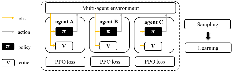
In IPPO, each agent uses the standard PPO sampling/training pipeline, making it a versatile baseline for multi-agent reinforcement learning tasks with reliable performance. It’s worth noting that the buffer and agent models can either be shared or trained separately across agents. This applies to all algorithms in the PPO family, not just IPPO.
Independent Proximal Policy Optimization (IPPO)#
Characteristic#
action space
|
|
task mode
|
|
|
|
taxonomy label
|
|
|
Insights#
In simpler terms, IPPO is a straightforward implementation of PPO for multi-agent reinforcement learning tasks. Each agent follows the same PPO sampling and training process, making it a versatile baseline for various MARL tasks. Unlike other MARL algorithms, IPPO does not require information sharing between agents, although it can still be optionally implemented for knowledge sharing.
Information Sharing
In the field of multi-agent learning, the term “information sharing” can be vague and unclear, so it’s important to provide clarification. We can categorize information sharing into three types:
real/sampled data: observation, action, etc.
predicted data: Q/critic value, message for communication, etc.
knowledge: experience replay buffer, model parameters, etc.
Traditionally, knowledge-level information sharing has been viewed as a “trick” and not considered a true form of information sharing in multi-agent learning. However, recent research has shown that knowledge sharing is actually crucial for achieving optimal performance. Therefore, we now consider knowledge sharing to be a valid form of information sharing in multi-agent learning.
Mathematical Form#
Standing at the view of a single agent, the mathematical formulation of IPPO is similiar as Proximal Policy Optimization: A Recap, except that in MARL, agent usually has no access to the global state typically under partial observable setting. Therefore, we use \(o\) for local observation and :math:`s`for the global state. We then rewrite the mathematical formulation of PPO as:
Critic learning: every iteration gives a better value function.
General Advantage Estimation: how good are current action regarding to the baseline critic value.
Policy learning: computing the policy gradient using estimated advantage to update the policy function.
\({\mathcal D}\) is the collected trajectories. \(R\) is the rewards-to-go. \(\tau\) is the trajectory. \(V_{\phi}\) is the critic function. \(A\) is the advantage. \(\gamma\) is discount value. \(\lambda\) is the weight value of GAE. \(u\) is the action. \(o\) is the local observation. \(\epsilon\) is a hyperparameter controlling how far away the new policy is allowed to go from the old. \(\pi_{\theta}\) is the policy function.
Note that in multi-agent settings, all the agent models can be shared, including:
critic function \(V_{\phi}\).
policy function \(\pi_{\theta}\).
Implementation#
We have made some modifications to the IPPO algorithm, specifically to the way the stochastic gradient descent (SGD) iteration is implemented. Other than that, we use the vanilla PPO implementation provided by RLlib as the basis for IPPO. You can find more information about the modifications we made to the SGD iteration in our documentation.
MultiGPUTrainOneSteplearn_on_loaded_batch
Key hyperparameter location:
marl/algos/hyperparams/common/ppomarl/algos/hyperparams/fintuned/env/ppo
MAPPO: PPO agent with a centralized critic#
Quick Facts
Multi-agent proximal policy optimization (MAPPO) is one of the extended version of IPPO: multi-agent version of PPO.
Agent architecture of MAPPO consists of two models:
policyandcritic.MAPPO is proposed to solve cooperative tasks but is still applicable to collaborative, competitive, and mixed tasks.
Preliminary:
Workflow#
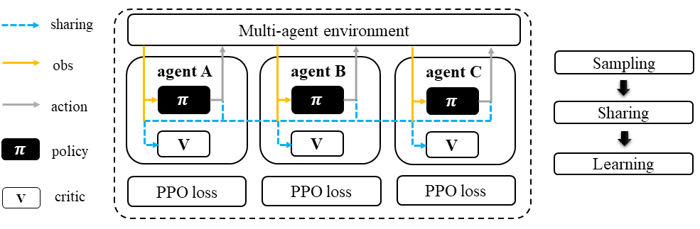
During the sampling stage in collaborative multi-agent reinforcement learning, agents need to communicate and share information with each other, such as observations and predicted actions. Once all the necessary information is collected, each agent follows the standard PPO training pipeline, but with the addition of a centralized value function for calculating the Generalized Advantage Estimation (GAE) and conducting the PPO critic learning procedure.
Multi-agent Proximal Policy Optimization (MAPPO)#
Characteristic#
action space
|
|
task mode
|
|
|
|
taxonomy label
|
|
|
Insights#
On-policy reinforcement learning algorithms are less sample efficient than their off-policy counterparts in MARL. The MAPPO algorithm overturn this consensus by experimentally proving that:
On-policy algorithms can achieve comparable performance to various off-policy methods.
MAPPO is a robust MARL algorithm for diverse cooperative tasks and can outperform SOTA off-policy methods in more challenging scenarios.
Formulating the input to the centralized value function is crucial for the final performance.
You Should Know
MAPPO paper is done in cooperative settings. Nevertheless, it can be directly applied to competitive and mixed task modes. Moreover, the performance is still good.
Sampling procedure of on-policy algorithms can be parallel conducted. Therefore, the actual time consuming for a comparable performance between MAPPO and off-policy algorithms is almost the same when we have enough sampling workers.
Parameters are shared across agents. Not sharing these parameters will not incur any problems. Conversely, partly sharing these parameters(e.g., only sharing the critic) can help achieve better performance in some scenarios.
Mathematical Form#
MAPPO needs information sharing across agents. Critic learning utilizes self-observation and information other agents provide, including observation and actions. Here we bold the symbol (e.g., \(u\) to \(\mathbf{u}\)) to indicate more than one agent information is contained.
Critic learning: every iteration gives a better centralized value function.
General Advantage Estimation: how good are current action regarding to the baseline critic value.
Policy learning: computing the policy gradient using estimated advantage to update the policy function.
Here \(\mathcal D\) is the collected trajectories that can be shared across agents. \(R\) is the rewards-to-go. \(\tau\) is the trajectory. \(A\) is the advantage. \(\gamma\) is discount value. \(\lambda\) is the weight value of GAE. \(u\) is the current agent action. \(\mathbf{u}^-\) is the action set of all agents, except the current agent. \(s\) is the global state. \(o\) is the local observation \(\epsilon\) is a hyperparameter controlling how far away the new policy is allowed to go from the old. \(V_{\phi}\) is the value function, which can be shared across agents. \(\pi_{\theta}\) is the policy function, which can be shared across agents.
Implementation#
Based on IPPO, we add centralized modules to implement MAPPO. The details can be found in:
centralized_critic_postprocessingcentral_critic_ppo_lossCC_RNN
Key hyperparameter location:
marl/algos/hyperparams/common/mappomarl/algos/hyperparams/fintuned/env/mappo
VDPPO: mixing a bunch of PPO agents’ critics#
Quick Facts
Value decomposition proximal policy optimization (VDPPO) is one of the extended version of IPPO: multi-agent version of PPO.
Agent architecture of VDPPO consists of three modules:
policy,critic, andmixer.VDPPO is proposed to solve cooperative and collaborative task modes.
Preliminary:
Workflow#
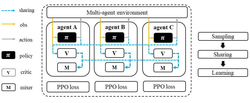
In the sampling stage, agents share information with others. The information includes others’ observations and predicted critic value. After collecting the necessary information from other agents, all agents follow the standard PPO training pipeline, except for using the mixed critic value to calculate the GAE and conduct the PPO critic learning procedure.
Value Decomposition Proximal Policy Optimization (VDPPO)#
Characteristic#
action space
|
|
task mode
|
|
taxonomy label
|
|
|
Insights#
VDPPO focuses on the credit assignment learning, which is similar to the joint Q learning family. VDPPO is easy to understand when you have basic idea of QMIX: mixing Q with monotonic factorization and VDA2C: mixing a bunch of A2C agents’ critics.
Mathematical Form#
VDPPO needs information sharing across agents. Therefore, the critic mixing utilizes both self-observation and other agents’ observation. Here we bold the symbol (e.g., \(u\) to \(\mathbf{u}\)) to indicate more than one agent information is contained.
Critic mixing: a learnable mixer for computing the global value function.
Critic learning: every iteration gives a better global value function.
General Advantage Estimation: how good are current joint action set regarding to the baseline critic value.
Policy learning: computing the policy gradient using estimated advantage to update the policy function.
Here \({\mathcal D}\) is the collected trajectories. \(R\) is the rewards-to-go. \(\tau\) is the trajectory. \(A\) is the advantage. \(\gamma\) is discount value. \(\lambda\) is the weight value of GAE. \(u\) is the current agent action. \(\mathbf{u}^-\) is the action set of all agents, except the current agent. \(s\) is the global state. \(o\) is the local observation. \(\epsilon\) is a hyperparameter controlling how far away the new policy is allowed to go from the old. \(V_{\phi}\) is the value function. \(\pi_{\theta}\) is the policy function. \(g_{\psi}\) is the mixer.
Implementation#
Based on IPPO, we add the mixer to implement VDPPO. The details can be found in:
value_mixing_postprocessingvalue_mix_ppo_surrogate_lossVD_RNN
Key hyperparameter location:
marl/algos/hyperparams/common/vdppomarl/algos/hyperparams/fintuned/env/vdppo
HAPPO: Sequentially updating critic of MAPPO agents#
Quick Facts
Heterogeneous-Agent Proximal Policy Optimisation (HAPPO) algorithm is based on MAPPO: PPO agent with a centralized critic.
Agent architecture of HAPPO consists of three modules:
policy,critic, andsequential updating.In HAPPO, agents have non-shared
policyand sharedcritic.HAPPO is proposed to solve cooperative and collaborative tasks.
Workflow#
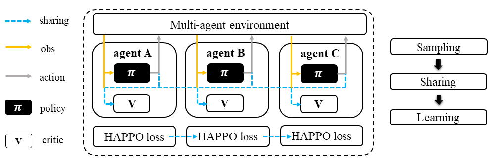
In the sampling stage, agents share information with others. The information includes others’ observations and predicted actions. After collecting the necessary information from other agents, all agents follow the standard PPO training pipeline, except HAPPO would update each policy sequentially. In this updating sequence, the next agent’s advantage is iterated by the current sampling importance and hte former advantage, except the first agent’s advantage is the original advantae value.
Heterogeneous-Agent Proximal Policy Optimization (HAPPO)#
Characteristic#
action space
|
|
task mode
|
|
taxonomy label
|
|
|
Insights#
Preliminary
The previous methods either hold the sharing parameters for different agents or lack the essential theoretical property of trust region learning, which is the monotonic improvement guarantee. This could lead to several issues when dealing with MARL problems. Such as:
If the parameters have to be shared, the methods could not apply to the occasions that different agents observe different dimensions.
Sharing parameters could suffer from an exponentially-worse suboptimal outcome.
although IPPO/MAPPO can be practically applied in a non-parameter sharing way, it still lacks the essential theoretical property of trust region learning, which is the monotonic improvement guarantee.
The HAPPO paper proves that for Heterogeneous-Agent:
Theoretically-justified trust region learning framework in MARL.
HAPPO adopts the sequential update scheme, which saves the cost of maintaining a centralized critic for each agent in CTDE(centralized training with decentralized execution).
Some Interesting Facts
A similar idea of the multi-agent sequential update was also discussed in dynamic programming, where artificial “in-between” states must be considered. On the contrary, HAPPO sequential update scheme is developed based on the paper proposed Lemma 1, which does not require any artificial assumptions and holds for any cooperative games
Bertsekas (2019) requires maintaining a fixed order of updates that is pre-defined for the task, whereas the order in MAPPO is randomised at each iteration, which also offers desirable convergence property
Mathematical Form#
Critic learning: every iteration gives a better value function.
Initial Advantage Estimation: how good are current action regarding to the baseline critic value.
Advantage Estimation for m = 1: how good are current action regarding to the baseline critic value of the first chosen agent.
Advantage Estimation if m > 1: how good are current action regarding to the baseline critic value of the chosen agent except the first one.
Policy learning: computing the policy gradient using estimated advantage to update the policy function.
Here \({\mathcal D}\) is the collected trajectories. \(R\) is the rewards-to-go. \(\tau\) is the trajectory. \(A\) is the advantage. \(\gamma\) is discount value. \(\lambda\) is the weight value of GAE. \(u\) is the current agent action. \(\mathbf{u}^-\) is the action set of all agents, except the current agent. \(s\) is the global state. \(o\) is the local information. \(\epsilon\) is a hyperparameter controlling how far away the new policy is allowed to go from the old. \(V_{\phi}\) is the value function. \(\pi_{\theta}\) is the policy function. \(B\) is batch size \(T\) is steps per episode
Implementation#
Based on MAPPO, we add three components to implement HAPPO. The details can be found in:
add_opponent_information_and_critical_vfhappo_surrogate_lossadd_all_agents_gae
Key hyperparameter location:
marl/algos/hyperparams/common/happomarl/algos/hyperparams/fintuned/env/happo